Get more out of system architectures
This case study shows how the evaluation of various design options requires a thorough approach to system-level modeling.
Developing complex systems requires extensive design reuse. Because of this reliance on reuse and also third party IP, you lose some of the flexibility of a custom RTL implementation; yet a benefit of leveraging IP is the latitude to experiment with different types and configurations. In this sense, the essential differentiation of a system lies in the efficient use of IP to build system architectures that best address the workload requirements of the target application.
This requires an accurate characterization of the different hardware implementation options based on software execution and workload characteristics. This article uses the example of a system design to look at some of the possible trade-offs and how a system can be quantitatively analyzed for a particular application. We have already used the design example in a test case and share some of the results below.
Architecture implementation alternatives
Our system handles data coming in through an Ethernet bridge. This data is processed and, based on a workload-appropriate response, sent back through the Ethernet bridge as well.
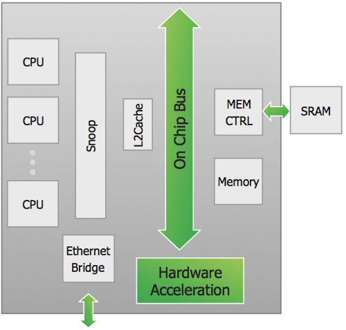
Figure 1
Example design (Source: Mentor Graphics – click image to enlarge)
In this design there are many architectural alternatives that can be explored to achieve an optimized implementation for a particular target market. Some of these include:
- The number of processing elements (CPUs)
- Cache attributes
- Sizing for both L1 and L2
- Shared versus dedicated cache
- Cache replacement algorithms
- Memory bandwidth
- Bus architecture
- Dedicated processor buses versus shared bus
- Layering and partitioning possibilities
- Hardware acceleration versus processor load
- Ethernet bandwidth
- Separate versus shared paths for input and output data
- Data processing path and resources
It is important to understand that it is impossible to determine the correct implementation by analyzing the hardware in isolation. The best choice of implementation can only be reached by taking the complete set of system characteristics into account. These include software processing, data transformation requirements, and the data flow in and out of the system.
To quantify our choices, you need an executable model of the system that can be manipulated to represent its function and performance based on the specific implementation options. The model needs to be accurate enough to allow you to properly compare alternatives and easy enough to create that you can afford to explore the architectural choices.
Generally RTL models are too detailed and too expensive for use in architectural trade-off analysis. The generally accepted method is to create a SystemC TLM2.0 approximately-timed (AT) transaction level model (Guide) of the architecture. This model is capable of running software and performing the data processing that will be done by the ultimate target system. It is also accurate enough to provide the quantitative performance feedback necessary.
Based on generic building blocks, specific IP blocks, and some custom models of the hardware accelerator, an initial model of our example platform was created in approximately two weeks. This model could easily be reconfigured to compare the different implementation choices listed above.
Data set description
The example system was targeted at an industrial automation and control application for which we had a very detailed understanding of the data flow requirements. We knew how much data would be coming into the system, what needed to be done to the data for the appropriate response actions, and how much data would be flowing out of the system. Thus we were able to create workload TLMs that could drive our model and be used to characterize the performance of different implementation options.
This analysis was done using SystemC TLM2.0 AT level models created using the Mentor Graphics Vista suite of tools. The work leveraged standard IP models available in the Vista libraries. The Vista suite was also used to automate the creation of the custom hardware accelerator model. Analysis information was extracted automatically, allowing very fast iteration and comparison of the alternatives.
We modeled more than 100 alternative architectures (number of CPUs, cache attributes, memory bandwidth, etc.). For example, we compared the tradeoffs between two architectural configurations (Case One and Case Two below) that would affect how incoming data was handled. Specifically, we evaluated an option for the hardware accelerator to analyze the data coming in through the Ethernet bridge. Based on the data type, the hardware accelerator could identify which portion was needed first by the CPU to perform its processing. This data could be pre-cached in the L1 of the appropriate processor to save memory subsystem access latency, bandwidth, and power. To achieve this, some additional intelligence had to be designed into the hardware accelerator inspecting the incoming data.
The flow of data in Case One:
- Data comes into the Ethernet Bridge; for other reasons, the data stream coming into the Ethernet bridge is visible to the hardware accelerator.
- The Ethernet bridge writes the data to SRAM.
- The hardware accelerator notifies one of the CPUs that the data is available to be processed.
- The CPU accesses the data in SRAM, performs its processing, and sends the appropriate messages back out of the system.
The flow of data in Case Two:
- Data comes into the Ethernet bridge.
- As the data arrives, the hardware accelerator determines if a portion of the data should be written directly to the L1 cache.
- The Ethernet bridge writes the data to the L1 cache and SRAM, as determined by the hardware accelerator.
- The hardware accelerator notifies one of the CPUs that the data is available to be processed.
- The CPU accesses the data; some portion of the data is already in the L1 cache; the rest of the data is retrieved from the SRAM as needed.
The hardware overhead for implementing the functionality in Case Two was relatively minor. The calculations to determine where the data was stored were ultimately done by either the CPU (Case One) or the hardware accelerator (Case Two). In terms of the implications for modeling, there was not a significant impact on the choice of where the calculations were performed; in fact, once the first case was created, the modification to implement the second case took less than half a day.
Description of results
Figures 2 and 3 plot the latency for each transaction from the CPUs to completely process a particular data set for the two cases. Both graphs show the processing of exactly the same workload. In both cases, exactly the same data transformation and responses were generated.
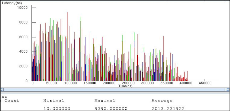
Figure 2
Latencies of transactions from the CPU (Case One) (Source: Mentor Graphics – click image to enlarge)
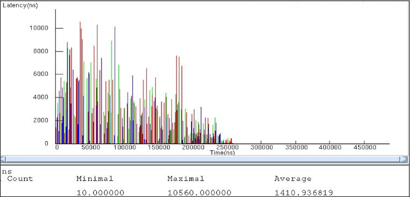
Figure 3
Latencies of transactions from the CPU (Case Two) (Source: Mentor Graphics – click image to enlarge)
The total time to process the data set was just over 400ms in the first case. This dropped to just over 250ms in the second case. The average service time dropped from over 2ms to 1.4ms. In other words, Case Two offered a 30% improvement in both total processing time and packet processing time. The cost of this improvement required moving a relatively small amount of processing from software to the hardware accelerator.
In addition to the performance benefit, the change also had a significant impact on the power consumed by the system. Below are the power graphs for both cases. The graphs track the power used by the memory subsystem and hardware accelerator only.
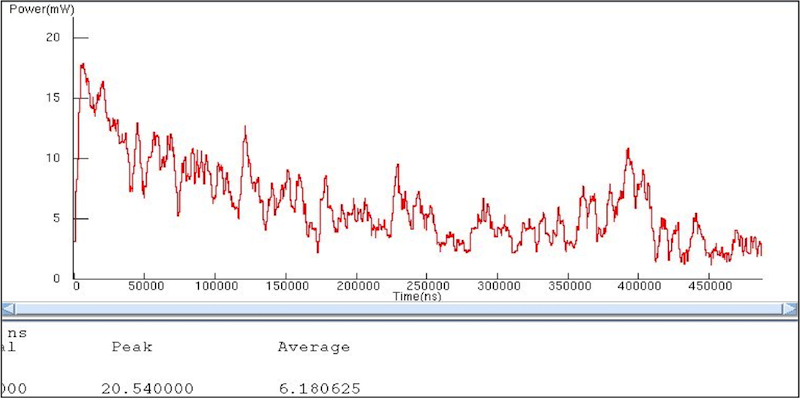
Figure 4
Dynamic power profile (Case One) (Source: Mentor Graphics – click image to enlarge)
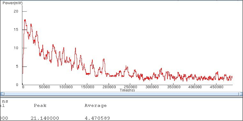
Figure 5
Dynamic power profile (Case Two) (Source: Mentor Graphics – click image to enlarge)
Again, Case Two gave us better power characteristics. The change in architecture led to a greater than 25% improvement in the power consumed by this portion of the system while increasing the performance of the entire system.
Conclusion
By modeling a system in SystemC at the TLM AT level, you can quickly characterize options and make informed decisions as to the best architecture to satisfy your system needs. As the importance of legacy RTL designs and third-party RTL IP increases, the value of system designs will be increasingly derived from improving how we select and architect the reused elements; thereby increasing the likelihood of delivering a successful solution for the target market and workload.
About the Author
Jon McDonald is Senior Technical Marketing Engineer at Mentor Graphics. He received a BS in Electrical and Computer Engineering from Carnegie Mellon University and an MS in Computer Science from Polytechnic University. He has been active in digital design, language based design and architectural modeling for over 15 years.
Contact
Mentor Graphics
Corporate Office
8005 SW Boeckman Rd
Wilsonville
OR 97070
USA
T: +1 800 547 3000
W: www.mentor.com