Antenna design considerations

An overview of antenna design considerations is presented. These considerations include system requirements, antenna selection, antenna placement, antenna element design/simulation and antenna measurements. A center-fed dipole antenna is presented as a design/simulation example. A measurement discussion includes reflection parameter measurements and directive gain measurements.

Antenna requirements

Gain and communication range

With the advent of prolific wireless communications applications, system designers are in a position to consider the placement and performance of an antenna system. The first step in establishing antenna requirements is to determine the desired communication range and terminal characteristics of the radio system (i.e., transmit power, minimum receiver sensitivity level). Given those parameters, one can ascertain the amount gain or loss required to maintain the communication range by using the Friis Transmission formula [1]:

where:

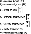
This relation is only valid for free-space propagation, but illustrates the important role of the antenna gain in the maximization of the receive-to-transmit power ratio, or system link gain.

Antenna size and clearance

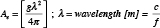
Antenna gain (or loss) must be part of a trade-off study between performance and the physical realization considerations of size, placement and clearance (distance from obstructions). One basic antenna relationship presented below shows that antenna gain, g, and then antenna effective aperture (area) are directly proportional. This roughly indicates that antenna gain is proportional to the physical size of the antenna [2].

Another basic antenna relationship shows the Fraunhofer or Rayleigh distance, d, at which the near/far-field transition zone exists. Ideally, there should be a free-space clearance zone around the antenna of at least d. The largest dimension of the antenna, D, and the operating wavelength determine this distance [3].

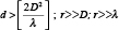
For example, if the largest dimension of the antenna is a half of a wavelength, the minimum clearance zone is a half-wavelength. This serves as a basic guideline, however in many physical realizations, this clearance zone is compromised and the effects must be determined through simulation or empirical measurement.

Antenna gain details

Antenna gain is defined as the ratio of radiated power intensity relative to the radiated power intensity of an isotropic (omni-directional) radiator. Power intensity is the amount of radiated power per unit solid angle measured in steradians (sr) [4]. The sphere associated with the isotropic radiator has a steradian measure of 4? steradians and serves as the normalization reference level for antenna gain.

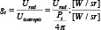
The antenna gain expression can be expanded further to reveal other factors that contribute to the overall antenna gain. The radiation intensity for the antenna is a function of the antenna efficiency, ?, and the directivity, D. The antenna efficiency is a product of the reflection efficiency or mismatch loss and the losses due to the finite resistances and losses in the antenna element conductor and dielectric structures. The mismatch loss can be ascertained through simulation or measurement of the antenna’s input impedance or reflection coefficient, ?. The directivity is a description of the gain variation as a function of the link axis angle(s) or the angle(s) of arrival/departure as described by the standard spherical coordinate system.

Antenna gain patterns

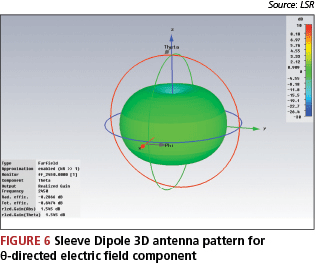
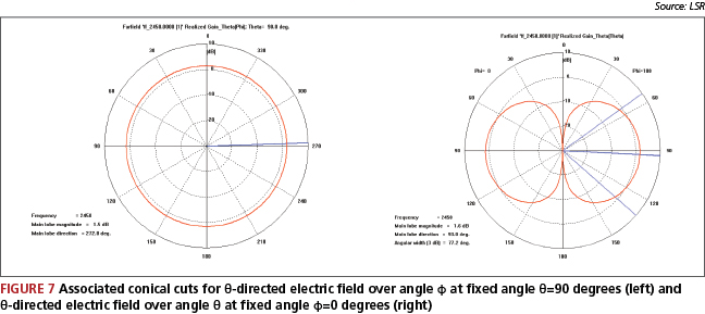
Ideally, antenna patterns are displayed as 3D plots (an example is shown to accompany the case study in Figure 6). The plot is often constructed from multiple cross sections known as conical cuts. A typical conical cut is formed by holding the elevation angle, ?, constant and measuring the pattern over a complete revolution of the azimuthal angle, ?. Secondly, a separate plot is generally made for each component of the electrical field or polarization (E?-horizontal or E?-vertical). Examples of conical cuts are presented in Figure 7, accompanying the case study.

Since most antenna patterns are not necessarily omni-directional, the description of antenna gain is fairly complex. In order to serve a system analysis in terms of determining communication range or system gain, the minimum, maximum and average gain over the entire pattern of a particular cut is typically used as the singular antenna gain value in the Friis transmission formula.

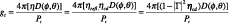
However, designers may want to determine the distribution of communication ranges and system gains, given the non-uniform nature of a directional antenna that is used in an omni-directional application. In those cases, probability density functions (pdfs) can be associated with antenna patterns, both conical cuts and 3D patterns [5]. Even though the directional antenna patterns are deterministic, the fact that their application is omni-directional with a random link axis angle makes the antenna gain a random variable with respect to communication range and system gain analyses. Figure 1 shows the pdf associated with both the omni- and non-uniform patterns presented on the left. On the right is the complementary-cumulative density function (ccdf), which is derived from the pdf and indicates the probability that the antenna can provide a minimum level of gain, given a random link axis angle.

Note for the case of the omni-directional antenna, the pdf is an impulse since the gain is single-valued and has no real distribution. The omni-directional case presents an interesting step-function ccdf. It shows that the probability of having a directive gain at least as large as the abscissa is 1 for gains less than the fixed gain value.

Antenna topologies

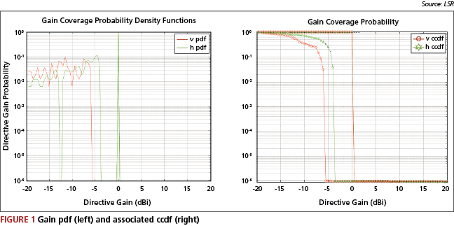
There are many possible topologies or structures for an antenna. One interesting set of structures is that which evolved from the basic half-wave dipole (Figure 2).

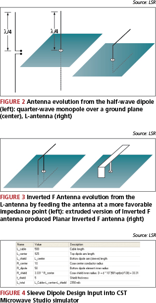
Starting with the half-wave dipole, the lower element of the dipole can be realized by a reflected image of the upper element onto a ground plane (using electric field boundary conditions and/or image theory). The monopole can be folded over, however, with degradation in impedance match and gain. The degradation due to matching can be recovered by feeding the antenna at a different point along the resonant length of the antenna (recall the impedance variation of a transmission line with a standing wave present). This results in the inverted ‘F’ antenna. The elements may be extruded from the wire form to a planar form to realize an increase in impedance and gain bandwidth, but with a small degradation in gain. These additional evolutions are presented in Figure 3.

Antenna design and simulation

The initial design of an antenna can arise from a set of dimensional formulas based on closed-form electromagnetic relations. In practice, however, these antennas require some empirical adjustment and/or tuning steps before you arrive at a final design. Secondly, the electromagnetic relations associated with most antennas are not of a closed form and therefore do not yield dimensional synthesis equations. Therefore, in order to design and validate an antenna prior to fabrication, it is worthwhile simulating the antenna using a electromagnetic field solver that can predict the behavior of radiating systems.

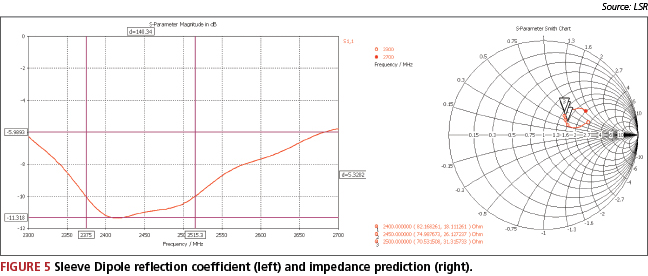
One such solver, CST Microwave Studio [6], offers many options that can simulate open-boundary, radiating structures. Figure 4 shows the relative utility of the simulation tool. It is the input page for a 2.4GHz sleeve dipole antenna, containing the dimensional and material parameter inputs required to carry out the simulation.

Upon completion of the electromagnetic simulation, the radiation pattern of the electric field is available as a 3D plot and as conical cuts. Further, the simulator predicts the input reflection coefficient and represents it as a scattering parameter (S11). The simulator provides all of the essential information about the antenna prior to its physical realization in order to pre-validate the design approach. The predicted reflection coefficient and driving point impedance are presented in Figure 5. The predicted 3D radiation pattern is presented in Figure 6, with associated conical cuts shown in Figure 7.

Antenna design validation and measurement

With the antenna synthesized and realized, the design must be validated through measurement. The first necessary measurement is to measure the reflection coefficient of the antenna input port or driving point. The reflection coefficient and associated driving point impedance is measured with a vector network analyzer (VNA). Care must be taken during this measurement to ensure that the antenna is radiating and not being disturbed by any surrounding objects. Ideally, this measurement is performed in an anechoic chamber. However, with sufficient separation between the antenna and any perturbing obstructions, this measurement can typically be performed within a normal laboratory environment.

In order to initially validate the antenna design, the reflection coefficient and associated driving point impedance must be such that the antenna is reasonably matched to the system impedance (generally 50?).

Once it has been established that the antenna is matched to the system impedance, the radiation pattern must be measured to complete the final steps of design validation. The measurements are performed in an anechoic chamber by exciting the antenna under test with a known transmit source power and measuring the received power, received voltage or electric field intensity at a fixed distance.

The antenna is swept through a series of conical cuts in an effort to compare them to simulated results or to build a set of cuts to assemble into a 3D gain pattern. The absolute received signal is normalized either by the conducted power applied to the antenna or compared to a known reference such as a half-wave dipole. Both polarization cases are measured. With the set of pattern data at hand, the measurements can also be examined against the system requirements in terms of minimum, maximum and average gain, or against gain distribution requirements, if applicable.

Conclusion

Antennas provide the primary interface between the radio and the propagation environment. The antenna requires special considerations in terms of performance requirements, design constraints, design and realization. Specification of the antenna gain and relating those requirements to the system performance in terms of range and system link gain is a foundation for the design goals of the antenna. During the antenna topology/structure selection process, consider packaging constraints in terms of the size, location and possible obstructions. Be prepared to compromise performance versus package conformance.

Ideally, one should use a simulation tool to assess the performance of the antenna prior to realization, not only to gauge the fundamental performance of the antenna, but also to check the effects of antenna compaction, obstructions and other compromised parameters. The final physical realization and consequent measurement of input terminal reflection/impedance and antenna gain complete the design process. Often, the measurement results require that the antenna structure be modified to empirically optimize its performance.

References

1. Harald Friis, “A Note on a Simple Transmission Formula,” Proc. IRE, 34, 1946, pp. 254-256.
2. Theile and Stutzman, Antenna Theory and Design, Second Edition, John Wiley and Sons, 1998, p. 79.
3. Theile and Stutzman, Antenna Theory and Design, Second Edition, John Wiley and Sons, 1998, p. 30.
4. Theile and Stutzman, Antenna Theory and Design, Second Edition, John Wiley and Sons, 1998, pp. 39-43.
5. B. Petted, “Antenna Gain Considerations in Communications System Range Analysis”, Seminar in Microwave Engineering, Marquette University, March 20, 2009.
6. CST Microwave Studio, CST of America, 492 Old Connecticut Path, Suite 505, Framingham, MA 01701. W: www.cst.com.

LS Research
W66 N220 Commerce Court
Cedarburg
WI 53012
USA

T: 1 262 375 4400
W: www.lsr.com